Data Collection through Bluetooth
|
The first step of the data collection would be Bluetooth connection establishment between WICED Sense and Android mobile phone. Broadcom WICED Sense™ Kit consists of a BCM20737L Bluetooth Low Energy System-on-Chip (SoC) and four STMicroelectronics sensors [5]. After Bluetooth connection establishment, WICED Sense would continuously send acceleration and gyroscope data to the Android phone per 100 milliseconds, so that the movement of exercise could be mapped to a digital signal and further could be detected and counted.
|

|
Real-time Data Pre-processing
Data Cleaning
|
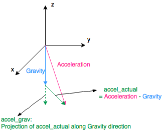
After collection of real-time data, the next step was data cleaning. To increase the accuracy of measurement, we focused on the movement signal in gravity direction. So, the first step of measurement was to find and update gravity. Gyroscope data assists us to update gravity, based on the assumption that if the gyroscope data was small enough, then the device was suspended. At this time, we would extract and interpret the gyroscope data as gravity. With gravity measured, we could have the actual acceleration during the movement by subtracting gravity from it. This process is shown in the figure on the left.
|
|
|
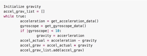
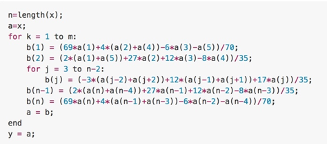
With actual acceleration measured, the final step of data cleaning was to multiply the actual acceleration with gravity, and this data was considered as a signal reflecting the exercise movement in gravity direction. The pseudocode is shown in pseudocode on the left.
|
|
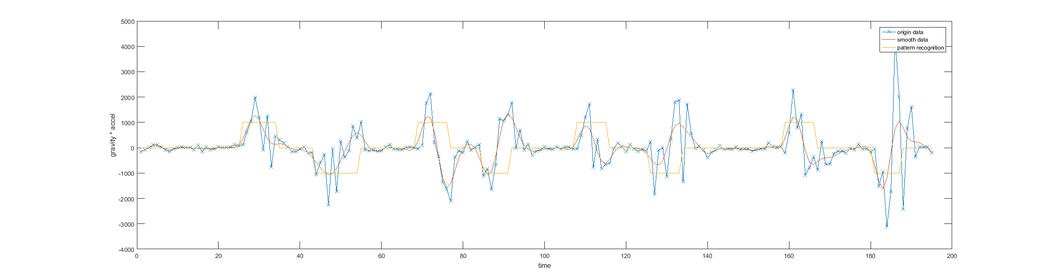
Fig 1. The Picture of Data Pre-processing. In the picture, the blue line showed origin data; the red line showed the data after smoothing; the yellow line showed the result of pattern recognition. There were four times of reciprocal movements, which were labelled by purple rectangle.
Data smoothing
|
The cleaned data was plotted as the blue line in Fig.1. We could see from this figure that the cleaned data was full of fluctuations; therefore, the next step was smoothing data to find the signal’s pattern. The method we used was called cubical smoothing algorithm with five-point approximation, and the pseudocode is shown on the left. The parameter m in pseudocode was the iteration time which was related to smooth performance, and we selected the iteration time parameter as 5 to get the smooth data in a window size of 5. The data after smoothing was shown as the red line in Fig.1. We could easily recognize each count in the signal’s pattern from this red line.
|
|
Pattern Recognition
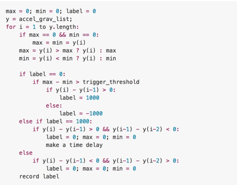
Final step was to count the exercise times according to the signal’s pattern. We founded that every period of the signal contains two pulses. One could be regarded as a rising edge-trigger and one as a falling edge-trigger. The physical meaning behind it was that, during the rising process of the reciprocating movement, the acceleration would increase to a maximum, and then gradually decrease to a negative minimum, and finally go back to zero when it reached the highest position. And the acceleration changed oppositely during the falling process of this reciprocating movement.
So we set up a threshold to find the rising and falling edge-trigger. When we found a rising trigger, we maintained high level output, until a crest of wave was detected. When we found a decreasing trigger, we maintained in low level output, until a peak of wave was detected. Between each trigger detection, we needed to wait for short time until the pulse finished. After processing data with this algorithm, we could find each exercise was detected as shown in the yellow line. We have indicated each reciprocation in a purple rectangle. The Pseudocode in this part is shown below.
So we set up a threshold to find the rising and falling edge-trigger. When we found a rising trigger, we maintained high level output, until a crest of wave was detected. When we found a decreasing trigger, we maintained in low level output, until a peak of wave was detected. Between each trigger detection, we needed to wait for short time until the pulse finished. After processing data with this algorithm, we could find each exercise was detected as shown in the yellow line. We have indicated each reciprocation in a purple rectangle. The Pseudocode in this part is shown below.
Recommendation Algorithm
|
In the recommendation part of our project, we used the collaborative filtering (CF) technique provided by the Scikit Learn [7] and PySpark [8] machine learning library. The reason why we chose CF is that although currently our data had only 9 features, in the future we want to take more and more user features and exercise sorts into consideration, thus as the feature matrix becomes large and sparse, CF would be the best choice.
User recommendation consisted of two parts: similar user recommendation and fitness plan recommendation. For similar user part, we first standardized the user matrix, then calculate the l2 pair-wise distance for each user, the nearest 10 users will be returned as the similar user recommendation result. For the fitness planning part, we implemented a user-based recommendation technique by using the ALS algorithm provided by Spark MLlib [8]. |

|
The idea behind this user-based recommendation is taking similar users’ preferences on certain items (exercises) to predict certain user’s choice of exercise. In a matrix factorization (MF) framework, MF optimizes:
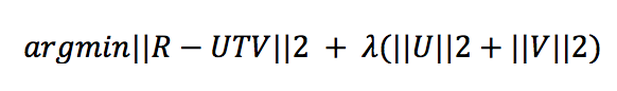
where partially represents the user-item preference matrix, and represent user and item feature factors separately. Solves least squares by initializing with average values and then keep fixed and optimize , and vice versa. The pseudocode of recommendation algorithm is shown below.
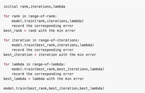
In this project, we first measured errors of different parameters with a small test dataset, and then choose the best combination of U and V automatically. Finally, we trained a model for the complete dataset to get final recommendations for every user.
Least Calories Consumed Estimation
we can estimate the least calories consumed based on the acquired fitness data and the basic information of the users, for example, age and weight.
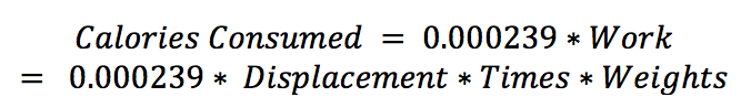
First, we translate the exercise data by multiplying physical displacement of the specific exercise “Displacement”, the counting times of the exercise “Times” and the weights of the plates on the exercise machine Weights. Therefore, we would have the total work done on the plates:
First, we translate the exercise data by multiplying physical displacement of the specific exercise “Displacement”, the counting times of the exercise “Times” and the weights of the plates on the exercise machine Weights. Therefore, we would have the total work done on the plates:

We had tested that for a 5.5 feet male, the estimated displacement of the exercise machine would be 60-80 cm per reciprocating movement. Therefore, we can translate the Work into calories consumed, where .
In this case, we could calculate the statistics of least calories consumed per every exercise. And the total estimation formula would be:
In this case, we could calculate the statistics of least calories consumed per every exercise. And the total estimation formula would be: